

Over the past few weeks US stock markets have been hitting record highs, leading many investors to wonder if it can continue and whether or not they need to be repositioning their portfolios, in the event that the party comes crashing down. There are many considerations, stretching from the AI trade running out of steam, to uncertainty about the underlying health of the US economy beyond the stock markets, to concerns around the direction of monetary policy, the Federal Reserve chair seemed to dampen expectations of any further rate cuts in 2025 having decided on just a -0.25% reduction in their recent October meeting.
To be clear there is never a one-size-fits-all solution to analyzing how an investment portfolio should be repositioned defensively in anticipation of a downturn but there are measures which some investors study to aid those decisions. In this instance we will choose to look at price-to-earnings (PE) ratios, a common rule of thumb to gauge whether its time to pivot from growth stocks to value stocks when there is a sense that the market is getting overheated. The +40 % ascent since the 2022 fall in the S&P 500 for instance, can squarely be placed on growth stocks, primarily tech driven AI with the addition of the booming AI infrastructure play.
Before introducing some PE figures to lend color to the current situation in the S&P 500 it is important to note, as most readers will be familiar with, that there are many variations on the theme of PE. From plain old current PE, trailing PE, forward looking PE up to the more elaborate versions like Robert Schiller’s cyclically smoothed CAPE. Often times, unfortunately, we are left looking at differing PE ratios for the same stocks or indices, with little reference to which of the many versions is being quoted. For the purposes of this quick analysis we shall be using current PE figures.
The normal process of using PE is to gauge the current level versus a chosen average, usually over a selected period that the individual investor decides reflects their given investment interests and horizons. Then based on the relative value compared to this average, the determination as to whether the stock or index in question is over or undervalued. This information is then used to assess the next course of action.
In our example we have used the S&P 500 index. See figure 1 by way of illustration. It uses data from 1998 to the present to incorporate the pre and post dotcom bubble, since some investors are worried that the AI trade may have some resemblance to it.
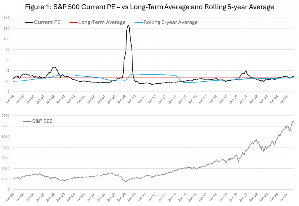
Observing the chart one can see that there are limitations that using the data. It is easy to draw inconsistent conclusions. Immediately it is clear that the long-term average whilst it might be interesting as a vague benchmark does not have any meaningful application to real world decisions. The rolling average however, appears to be more relevant.
Patterns can be found in the data, for instance when the Current PE level ascended above the Rolling 5-year Average in 2007 that looks like a good time to have left the market but can this observation be translated into a working system that worked on the basis of being in the market when the Rolling 5-year Average is higher than the Current PE? We should bear in mind, of course that this system is being built with the benefit of hindsight. To its credit though, a simple system such as this performs very well by comparison to doing nothing and remaining passively invested in the S&P 500, as is shown in Figure 2.
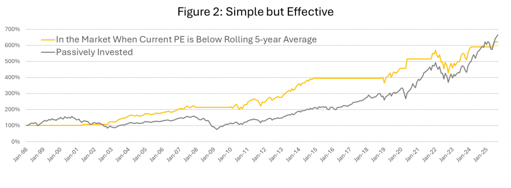
Yes, one would have missed the Dotcom boom and bust, yes one would have felt like a genius during the Great Financial Crisis, and yes one would also have avoided the worst of the Covid aberration. Furthermore, on balance over the long-term the cumulative return is a very respectable +621% vs +689% for the S&P 500. So a good strategy for an investor, but with the drawback of sitting making nothing while the market soars upwards, for example during the five years from 2014–2019.
Injecting More Context into PE Data
In our assessment using PE can be further assisted by vectorizing it. What do we mean by this? In physics, a vector is a quantity with magnitude and direction. In other words it represents a relationship between points. The Current PE we have used thus far is calculated as the Price per share divided by the most recent 12 months earnings per share (EPS). So in that sense both pieces of information are the most current data. That said however one, price is represented by a single point in time whereas EPS represents a range of time (12 months). This means that one could also look at a PE ratio, based on the price from at the time when the earnings range started. Looking forward at the earnings that were generated from the starting point price (historically speaking). When we then look at this figure in relation to its associated Current PE figure we have a relationship between two points. What this relationship allows us to do is to adjust for the movement of price within the PE ratio. Having these two points enables us to deduce both a magnitude and direction for one in relation to the other.
Figure 3 presents how this additional information can be used to create a simple systematic approach to determine when to be in, or out of the market.
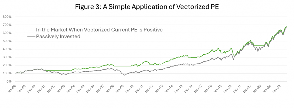
Beyond showing that it performs slightly better over the long-term than the S&P 500, it is clear that the this approach does not participate fully in the large market recoveries. Instead it performs with more consistency and less volatility by missing out on the dramatic falls thus losing less and being able to maintain its performance by compounding those returns, without having to dig itself out of a hole. More interestingly though is the difference between the Rolling 5-year Average model and the Vectorized PE model. They clearly are both protective but have a different patterns of returns. This leads to the conclusion that they can be used in conjunction with one another.
Improving the Tools for Investor Analysis
This brings us to Figure 4 which provides an illustration of how a systematic approach combining both models would perform relative to the S&P 500 over this same 27 year period. The combined model benefits hugely from retaining its invested capital and being able to capitalize on compounding those gains, as it captures the recovery upside, all be it still less vigorously than the index recovery.
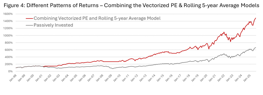
Ultimately this model achieves a very impressive more than two-fold return over the S&P 500, +1,539% vs +689% and it does this with a lower annualized volatility, 12.9% vs 15.4% for the S&P 500. It is of course far from perfect, for example, it remains in the market just like the passive, throughout the entirety of the decline in 2022. In conclusion it indicates that Vectorized PE can be quite easily applied to create sensible investment strategies. Some food for thought for investors as they try to assess the best market positions to adopt in the coming months. ■
© 2025 Plotinus Asset Management. All rights reserved.
Unauthorized use and/or duplication of any material on this site without written permission is prohibited.
Image Credit: Twin Design Studio at Shutterstock.